UFCFFY-15-M

Cyber Security Analytics

04: Machine Learning for Cyber Security

Prof. Phil Legg

04: Machine Learning for Cyber Security

In this session we will cover:

  • What is Machine Learning?
  • What different machine learning approaches are there?
  • How do we derive suitable features from our data, to then learn from?

What is Machine Learning?

A decision model that is not explicitly programmed, but instead is learnt through the training of example data.

Machine learning is an application of artificial intelligence (AI) that provides systems the ability to automatically learn and improve from experience without being explicitly programmed. Machine learning focuses on the development of computer programs that can access data and use it learn for themselves. We can essentially think of three components: an input (the data), a function, and an output.

The machine is trying to learn the function that can map inputs to some form of output, which is achieved by minimising some error measure (sometimes described as maximising a fitness function). One possible approach is to consider the difference between the expected output and the predicted output as the error measure - training is the process of iterative steps to reduce this measure.

Generative vs discriminative models

  • In generative models, given some input data the model will aim to generate new samples (e.g., deepfakes).
  • In discriminative models, given some input data the model will aim to discriminate between possible classes (e.g. classification).

Supervised Learning

This is where data is provided with training labels that inform the machine what the data is. For example, if we have a set of images that we wish to classify, we can state that the output is what the image depicts (for example, is it a cat or a dog?). The input to the system is the raw image data assessed based on colour pixel values. The output of the system is a label of either 'cat' or 'dog'. The function that converts the pixel input vector to a label output vector is what the machine attempts to learn. This is often described as classification.

Unsupervised Learning

This is where data is provided however no training labels are given. We want to learn some underlying properties about the data. Examples include clustering, where we aim to find hidden distributions within a larger set of data, association rules such as those used to identify shopping trends and similarities between consumer groups, and autoencoders that aim to learn suitable compression and decompression mechanisms for data representation and feature engineering.

Other forms of learning

  • semi-supervised (where we may inform the system only on a subset of samples, as identified through some means which could be unsupervised)
  • active learning (which involves a human-in-the-loop to label a small subset of data based on some underlying data attributes)
  • reinforcement learning (which is learning based on trial-and-error, popular for learning to play video games or robotic navigation)

Methods of Machine Learning
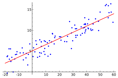
Linear Regression

  • Models linear relationship between a dependent variable (y, continuous output) and one or more explanatory (independent) variables (x, numercal input) - e.g., house prices, medical diagnosis, etc...
  • $y = m_0 + m_1 X$ (where $m_1$ are learnt weights for each $X$).
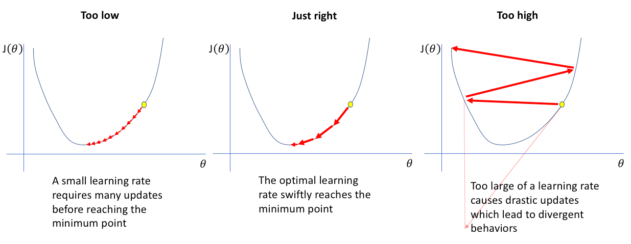
  • $m_0$ and $m_1$ learnt using Mean Square Error (MSE) and Gradient Descent.

More detail...

Alt text

In [11]:
#https://scikit-learn.org/stable/modules/generated/sklearn.linear_model.LinearRegression.html

import numpy as np
import matplotlib.pyplot as plt
from sklearn.linear_model import LinearRegression
X = np.array([ [1, 1], [1, 2], [2, 2], [2, 3] ])
#X = np.random.random([100,2])
y = np.dot(X, np.array([1, 2])) + 3
reg = LinearRegression().fit(X, y)
print ("X: ", X)
print ("y: ", y)
print ("Score: ", reg.score(X, y))
print ("Co-efficients: ", reg.coef_)
print ("Intecept: ",reg.intercept_)
print ("Prediction: ", reg.predict(np.array([[3, 5]])) )

#plt.scatter(X[:,0], X[:,1])
#plt.show()
X:  [[1 1]
 [1 2]
 [2 2]
 [2 3]]
y:  [ 6  8  9 11]
Score:  1.0
Co-efficients:  [1. 2.]
Intecept:  3.0000000000000018
Prediction:  [16.]
In [19]:
import matplotlib.pyplot as plt
import numpy as np

fig = plt.figure()
ax = fig.add_subplot(projection='3d')

xs = X[:,0]
ys = X[:,1]
zs = y
ax.scatter(xs, ys, zs)
ax.set_xlabel('X Label')
ax.set_ylabel('Y Label')
ax.set_zlabel('Z Label')
plt.show()

Clustering

  • Unsupervised approach to find similar datapoints and uncover hidden distributions (e.g., malware families, or malicious v benign).
  • k-means clustering - identify $k$ unique clusters based on group centroid (mean).

More detail...

Alt text

In [9]:
# https://scikit-learn.org/stable/modules/generated/sklearn.cluster.KMeans.html

import numpy as np
import matplotlib.pyplot as plt
from sklearn.cluster import KMeans

X = np.array([[1, 2], [1, 4], [1, 0], [10, 2], [10, 4], [10, 0]])
kmeans = KMeans(n_clusters=2, random_state=42).fit(X)
print ("Labels: ", kmeans.labels_)#
print ("Predictions: ", kmeans.predict([[0, 0], [12, 3]]) )
print ("Centroids: ", kmeans.cluster_centers_)

plt.scatter(X[:,0], X[:,1])
plt.show()
Labels:  [1 1 1 0 0 0]
Predictions:  [1 0]
Centroids:  [[10.  2.]
 [ 1.  2.]]

Support Vector Machines

  • Supervised approach to identify decision boundary between clusters (unlike LR that fits a line through points).
  • Measure euclidean distance between data points nearest to the decision boundary and the boundary.
  • Optimise the distance of the points from the boundary.

More detail...

In [14]:
# https://scikit-learn.org/stable/modules/svm.html

from sklearn import svm
X = np.array([[0, 0], [1, 1]])
y = np.array([0, 1])
clf = svm.SVC()
clf.fit(X, y)
print ("Prediction: ", clf.predict(np.array([[2., 2.]])))

plt.scatter(X[:,0], X[:,1])
plt.show()
Prediction:  [1]

Dimensionality Reduction

  • Principal Component Analysis (PCA) is a common approach (also t-SNE, UMAP)- reduce the dimensionality but preserve the data structure (separability/distance between points).
  • Data compression and aids visualisation using projection view.
  • For a given dataset, PCA finds directions (or vector) of greatest variance - the principal components - used as new axis in $N-1$ space.

More detail...

In [50]:
# https://scikit-learn.org/stable/modules/generated/sklearn.decomposition.PCA.html
# https://scikit-learn.org/stable/auto_examples/cluster/plot_kmeans_digits.html

import numpy as np
import matplotlib.pyplot as plt
from sklearn.datasets import load_digits

data, labels = load_digits(return_X_y=True)
(n_samples, n_features), n_digits = data.shape, np.unique(labels).size

print("Original data: #digits:", n_digits, " #samples:", n_samples, " #features:", n_features)
sample = 10
plt.imshow(data[sample,:].reshape(8,8))
plt.show()
print("Label: ", labels[sample])
Original data: #digits: 10  #samples: 1797  #features: 64
Label:  0
In [51]:
from sklearn.decomposition import PCA
pca = PCA(n_components=2)
result = pca.fit_transform(data)
print ("Shape: ", result.shape)
plt.scatter(result[:,0], result[:,1], c=labels)
# plt.scatter(result[sample,0], result[sample,1], s=200, marker='X', color='red') - show sample in cluster
plt.show()
Shape:  (1797, 2)

Neural Networks

  • Maps input vector to output vector through matrix multiplication of weighting functions.
  • Feed-forward network: $y = sigmoid (Wx + b)$
  • How to resolve error? Backpropagation used to minimise distance between the predicted values and our expected values - the process of "training" the neural network.

More detail...

In [57]:
# https://scikit-learn.org/stable/modules/generated/sklearn.neural_network.MLPClassifier.html

from sklearn.neural_network import MLPClassifier
from sklearn.datasets import make_classification
from sklearn.model_selection import train_test_split
X, y = make_classification(n_samples=100, random_state=1)
X_train, X_test, y_train, y_test = train_test_split(X, y, stratify=y, random_state=42)
clf = MLPClassifier(random_state=1, max_iter=300).fit(X_train, y_train)
print ("Prediction (Probability): ", clf.predict_proba(X_test[:1]))
print ("Prediction (Class Label): ", clf.predict(X_test[:5, :]))
print ("Accuracy: ", clf.score(X_test, y_test))
Prediction (Probability):  [[0.00415509 0.99584491]]
Prediction (Class Label):  [1 1 1 0 1]
Accuracy:  0.96

Feature Engineering

How should we present data to a classifier?

  • Images/Video: Pixel data
  • PCAP: Src? Dest? Port? Protocol? No single right answer...
  • Files: File size? Ordered bytes? Process calls? Anything else?

What about sequential data such as text?

  • n-grams: sliding window of $n$-items in data (e.g. 'The cat', 'cat sat', 'sat on', 'on the', 'the mat'). Count occurrence of $n$ ordered entities. Can be used at word or character level.

More on Statistical Analysis - SDAV

More on Text Analytics - SDAV

More on Text Analysis

  • https://chat.openai.com/chat
  • https://en.wikipedia.org/wiki/BERT_(language_model)
  • https://scikit-learn.org/stable/tutorial/text_analytics/working_with_text_data.html
  • https://pypi.org/project/transformers/
  • Ashish Vaswani, Noam Shazeer, Niki Parmar, Jakob Uszkoreit, Llion Jones, Aidan N. Gomez, Lukasz Kaiser, Illia Polosukhin. "Attention Is All You Need" NIPS, 2017

Further Reading

  • M. A. Ayub, S. Smith, A. Siraj and P. Tinker, "Domain Generating Algorithm based Malicious Domains Detection," 2021 8th IEEE International Conference on Cyber Security and Cloud Computing (CSCloud)
  • Daniele Ucci, Leonardo Aniello and Roberto Baldoni, "Survey of machine learning techniques for malware analysis" Computers and Security, Volume 81, March 2019, Pages 123-147
  • Andrew Y. Ng and Michael I. Jordan. "On Discriminative vs. Generative classifiers: A comparison of logistic regression and naive Bayes" Advances in Neural Information Processing Systems, 2002
  • M. Rhode, P. Burnap and K. Jones, “Early-stage malware prediction using recurrent neural networks”. Computers & Security, Volume 77, August 2018, Pages 578-594.
  • A. Mills, T. Spyridopoulos and P. Legg, “Efficient and Interpretable Real-Time Malware Detection Using Random-Forest,” 2019 International Conference on Cyber Situational Awareness, Data Analytics And Assessment (Cyber SA), 2019, pp. 1-8, doi: 10.1109/CyberSA.2019.8899533.

Practical Session

  1. Try the 04-Machine Learning lab examples
  2. Explore the scikit-learn library library
  3. Release of Assignment Portfolio Task 2