In this lab we will experiment with some small Machine Learning examples. We will draw on some common examples, including some from the scikit-learn documentation. You are encouraged to investigate scikit-learn further to develop your understanding of classification, clustering, supervised, and unsupervised learning.
The purpose of this lab is to help you understand some existing Machine Learning examples, and to get hands-on with running the code samples, and studying what the code is doing at each stage. You may choose to look at the examples in any order, based on the appeal of the activity.
Useful Resources:
The MNIST digit classification is a classic ML example, consisting of 60,000 labeled images of digits between 0 and 9. Each image is a 8x8 grayscale image, that we treat as an array.
Full details of this example available here: https://scikit-learn.org/stable/auto_examples/classification/plot_digits_classification.html#sphx-glr-auto-examples-classification-plot-digits-classification-py
import matplotlib.pyplot as plt
# Import datasets, classifiers and performance metrics
from sklearn import datasets, svm, metrics
from sklearn.model_selection import train_test_split
digits = datasets.load_digits()
_, axes = plt.subplots(nrows=1, ncols=4, figsize=(10, 3))
for ax, image, label in zip(axes, digits.images, digits.target):
ax.set_axis_off()
ax.imshow(image, cmap=plt.cm.gray_r, interpolation="nearest")
ax.set_title("Training: %i" % label)
Recall that a single data instance is made up of a set of features. We can think of this as a data instance being a 'row' in a DataFrame, and the set of features being each 'column'.
How do we then adapt images to fit this idea?
We can flatten the image, so that the 2D 8x8 array becomes a 1x64 array. Then, the entire dataset will be of shape (n_samples, n_features), where n_samples is the number of images and n_features is the total number of pixels in each image.
We can then split the data into train and test subsets and fit a support vector classifier on the train samples. The fitted classifier can subsequently be used to predict the value of the digit for the samples in the test subset.
# flatten the images
n_samples = len(digits.images)
data = digits.images.reshape((n_samples, -1))
# Create a classifier: a support vector classifier
clf = svm.SVC(gamma=0.001)
# Split data into 50% train and 50% test subsets
X_train, X_test, y_train, y_test = train_test_split(
data, digits.target, test_size=0.5, shuffle=False
)
# Learn the digits on the train subset
clf.fit(X_train, y_train)
# Predict the value of the digit on the test subset
predicted = clf.predict(X_test)
_, axes = plt.subplots(nrows=1, ncols=4, figsize=(10, 3))
for ax, image, prediction in zip(axes, X_test, predicted):
ax.set_axis_off()
image = image.reshape(8, 8)
ax.imshow(image, cmap=plt.cm.gray_r, interpolation="nearest")
ax.set_title(f"Prediction: {prediction}")
print(
f"Classification report for classifier {clf}:\n"
f"{metrics.classification_report(y_test, predicted)}\n"
)
Classification report for classifier SVC(gamma=0.001): precision recall f1-score support 0 1.00 0.99 0.99 88 1 0.99 0.97 0.98 91 2 0.99 0.99 0.99 86 3 0.98 0.87 0.92 91 4 0.99 0.96 0.97 92 5 0.95 0.97 0.96 91 6 0.99 0.99 0.99 91 7 0.96 0.99 0.97 89 8 0.94 1.00 0.97 88 9 0.93 0.98 0.95 92 accuracy 0.97 899 macro avg 0.97 0.97 0.97 899 weighted avg 0.97 0.97 0.97 899
disp = metrics.ConfusionMatrixDisplay.from_predictions(y_test, predicted)
disp.figure_.suptitle("Confusion Matrix")
print(f"Confusion matrix:\n{disp.confusion_matrix}")
plt.show()
Confusion matrix: [[87 0 0 0 1 0 0 0 0 0] [ 0 88 1 0 0 0 0 0 1 1] [ 0 0 85 1 0 0 0 0 0 0] [ 0 0 0 79 0 3 0 4 5 0] [ 0 0 0 0 88 0 0 0 0 4] [ 0 0 0 0 0 88 1 0 0 2] [ 0 1 0 0 0 0 90 0 0 0] [ 0 0 0 0 0 1 0 88 0 0] [ 0 0 0 0 0 0 0 0 88 0] [ 0 0 0 1 0 1 0 0 0 90]]
Reflect on the above code cells, and see what happens when you change aspects of this. For example, what if your train/test split was different? What if you use a different classifier rather than SVC?
Also, what does the classification report tell you? What does the confusion matrix tell you?
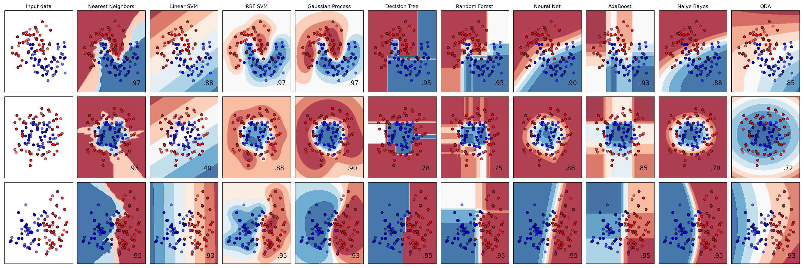
A comparison of a several classifiers in scikit-learn on synthetic datasets. The point of this example is to illustrate the nature of decision boundaries of different classifiers. This should be taken with a grain of salt, as the intuition conveyed by these examples does not necessarily carry over to real datasets.
Particularly in high-dimensional spaces, data can more easily be separated linearly and the simplicity of classifiers such as naive Bayes and linear SVMs might lead to better generalization than is achieved by other classifiers.
The plots show training points in solid colors and testing points semi-transparent. The lower right shows the classification accuracy on the test set.
### COPY IN THE CODE SAMPLE FROM THE LINK ABOVE TO SEE THIS IN ACTION
Why is this important for Machine Learning? Understanding how decision boundaries are defined is crucial for the separation of two or more classes, in a classification task. Understanding that some samples will be well within a class, whilst some may be situated closer to the boundary is important as it shows a level of confidence about how the classification is made, and it also shows some inherent characteristics of the data instance.
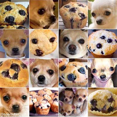
For example, think about a dog/cat classification tool. Some cases will be very obvious whilst others may be much more subtle and so will naturally sit at the decision boundary. Another classic example to illustrate this is the Chihuahua or muffin Internet meme - more details here.
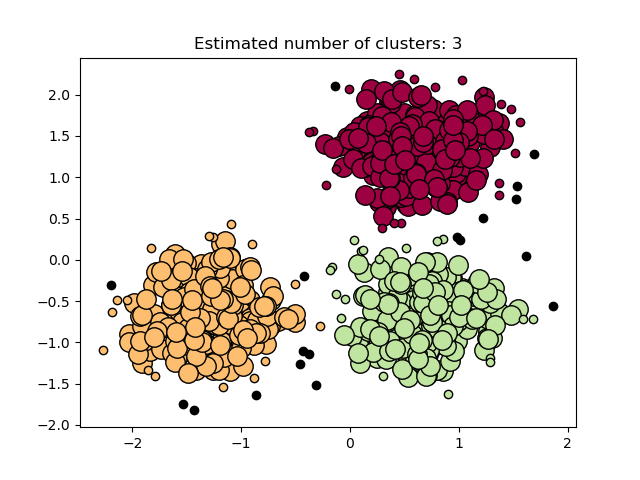
DBSCAN (Density-Based Spatial Clustering of Applications with Noise) finds core samples in regions of high density and expands clusters from them. This algorithm is good for data which contains clusters of similar density.
See the Comparing different clustering algorithms on toy datasets example for a demo of different clustering algorithms on 2D datasets.
Clustering is a powerful technique for finding similarities between instances. It is an unsupervised approach to learning some inherent groupings within a large dataset, without explicitly having to define what classes exist.
### COPY IN THE CODE SAMPLE FROM THE LINK ABOVE TO SEE THIS IN ACTION
In this example, semi-supervised classifiers are trained on the 20 newsgroups dataset (which will be automatically downloaded).
You can adjust the number of categories by giving their names to the dataset loader or setting them to None to get all 20 of them.
import numpy as np
from sklearn.datasets import fetch_20newsgroups
from sklearn.feature_extraction.text import CountVectorizer
from sklearn.feature_extraction.text import TfidfTransformer
from sklearn.preprocessing import FunctionTransformer
from sklearn.linear_model import SGDClassifier
from sklearn.model_selection import train_test_split
from sklearn.pipeline import Pipeline
from sklearn.semi_supervised import SelfTrainingClassifier
from sklearn.semi_supervised import LabelSpreading
from sklearn.metrics import f1_score
# Loading dataset containing first five categories
data = fetch_20newsgroups(
subset="train",
categories=[
"alt.atheism",
"comp.graphics",
"comp.os.ms-windows.misc",
"comp.sys.ibm.pc.hardware",
"comp.sys.mac.hardware",
],
)
print("%d documents" % len(data.filenames))
print("%d categories" % len(data.target_names))
print()
# Parameters
sdg_params = dict(alpha=1e-5, penalty="l2", loss="log")
vectorizer_params = dict(ngram_range=(1, 2), min_df=5, max_df=0.8)
# Supervised Pipeline
pipeline = Pipeline(
[
("vect", CountVectorizer(**vectorizer_params)),
("tfidf", TfidfTransformer()),
("clf", SGDClassifier(**sdg_params)),
]
)
# SelfTraining Pipeline
st_pipeline = Pipeline(
[
("vect", CountVectorizer(**vectorizer_params)),
("tfidf", TfidfTransformer()),
("clf", SelfTrainingClassifier(SGDClassifier(**sdg_params), verbose=True)),
]
)
# LabelSpreading Pipeline
ls_pipeline = Pipeline(
[
("vect", CountVectorizer(**vectorizer_params)),
("tfidf", TfidfTransformer()),
# LabelSpreading does not support dense matrices
("todense", FunctionTransformer(lambda x: x.todense())),
("clf", LabelSpreading()),
]
)
def eval_and_print_metrics(clf, X_train, y_train, X_test, y_test):
print("Number of training samples:", len(X_train))
print("Unlabeled samples in training set:", sum(1 for x in y_train if x == -1))
clf.fit(X_train, y_train)
y_pred = clf.predict(X_test)
print(
"Micro-averaged F1 score on test set: %0.3f"
% f1_score(y_test, y_pred, average="micro")
)
print("-" * 10)
print()
if __name__ == "__main__":
X, y = data.data, data.target
X_train, X_test, y_train, y_test = train_test_split(X, y)
print("Supervised SGDClassifier on 100% of the data:")
eval_and_print_metrics(pipeline, X_train, y_train, X_test, y_test)
# select a mask of 20% of the train dataset
y_mask = np.random.rand(len(y_train)) < 0.2
# X_20 and y_20 are the subset of the train dataset indicated by the mask
X_20, y_20 = map(
list, zip(*((x, y) for x, y, m in zip(X_train, y_train, y_mask) if m))
)
print("Supervised SGDClassifier on 20% of the training data:")
eval_and_print_metrics(pipeline, X_20, y_20, X_test, y_test)
# set the non-masked subset to be unlabeled
y_train[~y_mask] = -1
print("SelfTrainingClassifier on 20% of the training data (rest is unlabeled):")
eval_and_print_metrics(st_pipeline, X_train, y_train, X_test, y_test)
print("LabelSpreading on 20% of the data (rest is unlabeled):")
eval_and_print_metrics(ls_pipeline, X_train, y_train, X_test, y_test)
2823 documents 5 categories Supervised SGDClassifier on 100% of the data: Number of training samples: 2117 Unlabeled samples in training set: 0 Micro-averaged F1 score on test set: 0.905 ---------- Supervised SGDClassifier on 20% of the training data: Number of training samples: 426 Unlabeled samples in training set: 0 Micro-averaged F1 score on test set: 0.737 ---------- SelfTrainingClassifier on 20% of the training data (rest is unlabeled): Number of training samples: 2117 Unlabeled samples in training set: 1691 End of iteration 1, added 1084 new labels. End of iteration 2, added 210 new labels. End of iteration 3, added 61 new labels. End of iteration 4, added 17 new labels. End of iteration 5, added 16 new labels. End of iteration 6, added 4 new labels. End of iteration 7, added 4 new labels. End of iteration 8, added 1 new labels. End of iteration 9, added 2 new labels. End of iteration 10, added 3 new labels. Micro-averaged F1 score on test set: 0.807 ---------- LabelSpreading on 20% of the data (rest is unlabeled): Number of training samples: 2117 Unlabeled samples in training set: 1691
C:\Users\pa-legg\Anaconda3\lib\site-packages\sklearn\utils\validation.py:593: FutureWarning: np.matrix usage is deprecated in 1.0 and will raise a TypeError in 1.2. Please convert to a numpy array with np.asarray. For more information see: https://numpy.org/doc/stable/reference/generated/numpy.matrix.html warnings.warn( C:\Users\pa-legg\Anaconda3\lib\site-packages\sklearn\utils\validation.py:593: FutureWarning: np.matrix usage is deprecated in 1.0 and will raise a TypeError in 1.2. Please convert to a numpy array with np.asarray. For more information see: https://numpy.org/doc/stable/reference/generated/numpy.matrix.html warnings.warn(
Micro-averaged F1 score on test set: 0.667 ----------
For this task, we will focus on Cats Vs Dogs (since I tend to always use this example in the lectures!)
The blog Machine Learning Mastery by Jason Brownlee provides a very detailed breakdown of this task: How to Classify Photos of Dogs and Cats (with 97% accuracy)
The dataset used is available from Kaggle: Dogs Vs Cats Dataset
The dataset and task is part of the academic paper Asirra: A CAPTCHA that Exploits Interest-Aligned Manual Image Categorization by Elson et al., published in the Proceedings of 14th ACM Conference on Computer and Communications Security (CCS), 2007 - one of the leading cyber security academic conferences globally!
The blog article uses the Keras library, and Convolution Neural Networks, which are designed specifically to learn about patterns and spatial structures from image data. This is more challenging than using the scikit-learn, however would give you an appreciation of how more complex data types can be used to inform a classifier.
# USE THIS CELL FOR YOUR CODE SAMPLES
The last example we discuss here is on time series forecasting. So far, all data instances or observations have been independent (i.e., no explicit ordering of the data). In some applications however, time ordering will be crucial (e.g., behavioural change of a system or of a software executable).
The blog post ML Approaches for Time Series by Pablo Ruiz on Towards Data Science provides useful information, as does the time series analysis guide on Kaggle.
# USE THIS CELL FOR YOUR CODE SAMPLES